Abstract
We propose a new approach for modeling connector insertion environments by learning a quasi-static contact force model instead of a full simulator. Using a feature vector that contains information about the configuration and control, we find a linear mapping adequately captures the relationship between this feature vector and the sensed contact forces. A novel Linear Model Learning (LML) algorithm is used to solve for the globally optimal mapping in real time without any matrix inversions, resulting in an algorithm that runs in nearly constant time on a GPU as the model size increases. We validate the proposed approach for connector insertion both in simulation and hardware experiments, where the learned model is combined with an optimization-based controller to achieve smooth insertions in the presence of misalignments and uncertainty.
Feature-Based Contact Force Model
We are learning a model that maps an engineered feature vector, $w \in \mathbf{R}^{n_w}$, to the predicted force torque sensor, $\hat{y} \in \mathbf{R}^6$. The feature vector is a function of the configuration $q \in \mathbf{R}^{n_q}$, and the control $u \in \mathbf{R}^{n_u}$, and is defined as the following: $$ w = \Omega(q, u). $$ We then map this feature vector to the force torque sensor with a matrix $G$: $$ \hat{y} = Gw. $$ This model is learned online with by solving the following optimization problem: $$ \min_G \quad \sum_{i=1}^N \color{blue}{\underbrace{\color{black}{\| y_i - Gw_i \|_{R^{-1}}^2}}_{\text{model error}}} \color{black}{+} \color{red}{\underbrace{\color{black}{\| G b\|_2^2}}_{\text{regularizer}}} \color{black}{,} $$ where $R \in \mathbf{S}_+^{6}$ is the force torque sensor noise covariance, and $b \in \mathbf{R}^{n_w}$ is a regularization term. Even when the feature vector is nonlinear in $q$ and $u$, this is still a convex optimization problem that we can solve to global optimality.
Linear Model Learning (LML) Algorithm
This optimization problem is solved with a fast and parallelizable novel LML algorithm that updates the model in real time as new measurements come in. The LML algorithm maintains a Gaussian belief of the model parameters $\hat{G} \in \mathbf{R}^{6 \times n_w}$, with a shared covariance $\Sigma \in \mathbf{S}_+^{n_w \times n_w}$.
This belief is initialized with the regularization terms, as the following: $$\begin{align} \hat{G}_{0|0} &= 0, \quad \quad \quad \quad \quad & \Sigma_{0|0} &= \operatorname{diag}(1 / b^2), \nonumber \end{align}$$ and each time a new measurement and feature vector is available, the LML algorithm is called to update this belief:
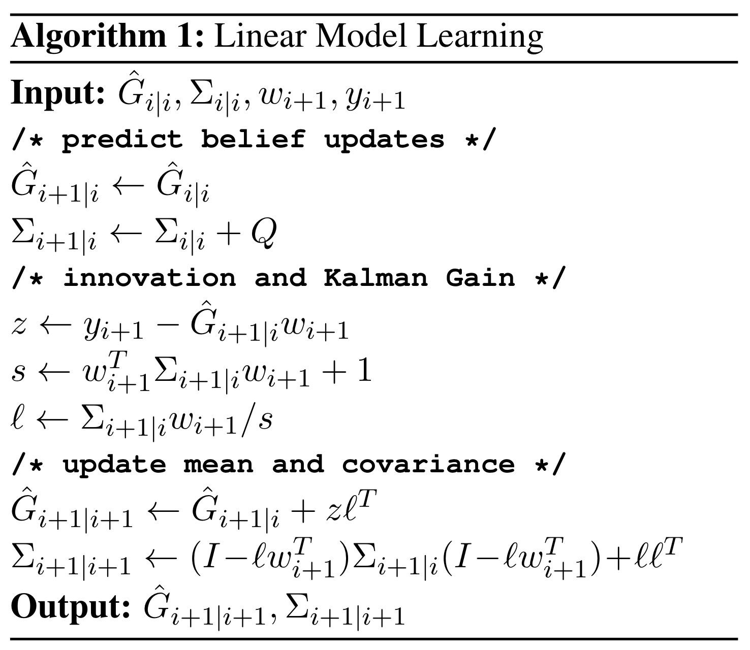
This algorithm is entirely free of matrix inversions, meaning each operation is highly parallelizable on a GPU. As a result, the LML algorith scales extremeley well as the complexity of the model increases. To demonstrate this, we show the runtime of the LML algorithm on a CPU and GPU as the sensor dimension and feature vector dimension increase.
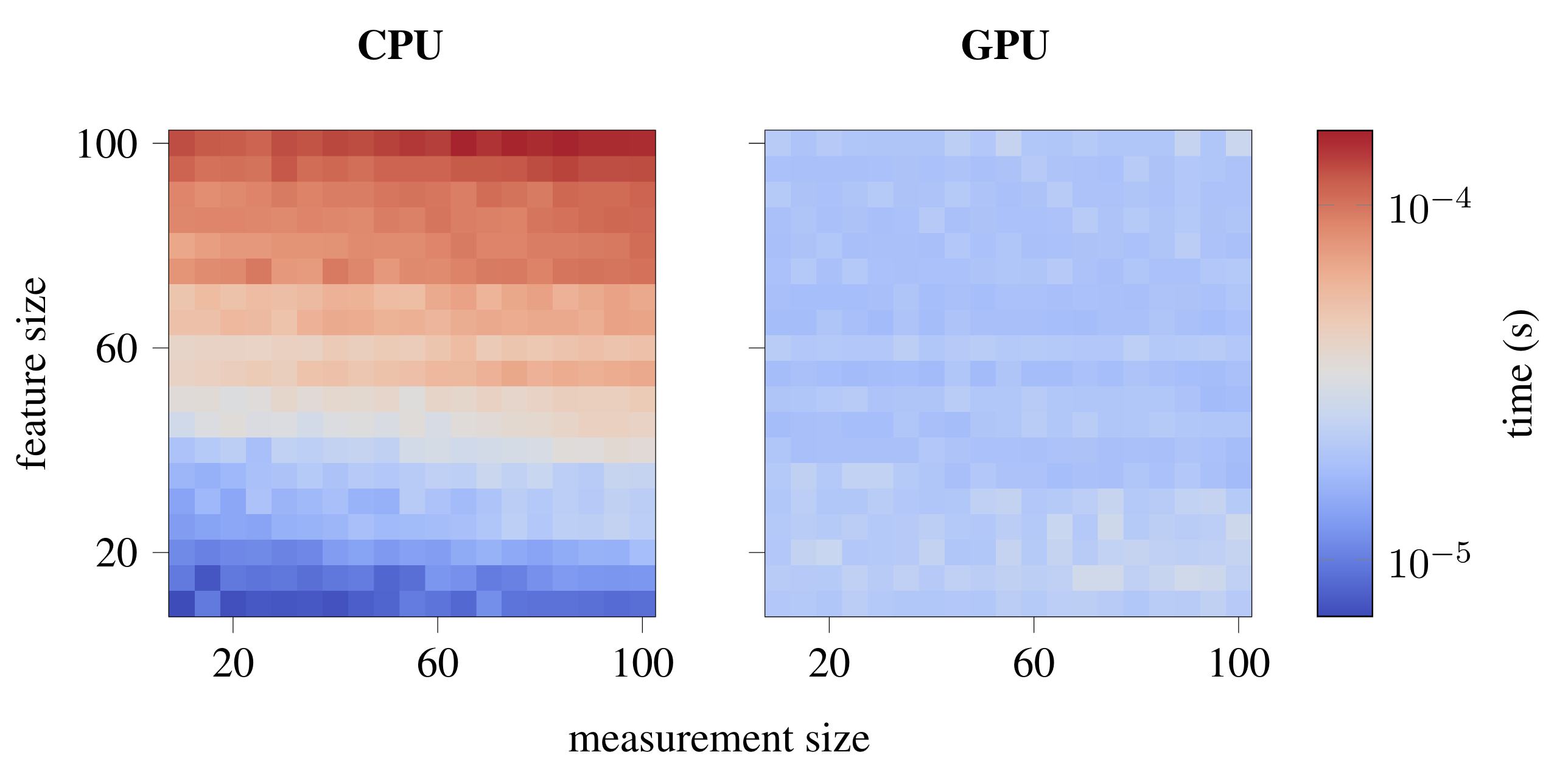
CPU and GPU runtimes as the LML algorithm is run for various sensor/feature sizes. Despite the number of parameters in the model growing by a factor of 100, the GPU is able to run LML in nearly constant time.
Experiments
To validate the ideas presented in this paper, we performed experiments in both simulation and on hardware. A full tutorial of our approach is demonstrated in MuJoCo in the colab link above. The LML algorithm is used with a straightforward feature vector to match the force torque sensor data from MuJoCo, after which this model is used in model-based controller that is able to successfuly insert the connector without any added resistance. This example is shown in the video at the top of this page.
We also performed experiments on hardware where an impedance-controlled Franka Panda robot with a parallel gripper was able to insert C13 power plugs. First, the validity of our linear model assumption is shown during a calibration sequence, where the real force torque sensor data is compared to the predicted values from our model:
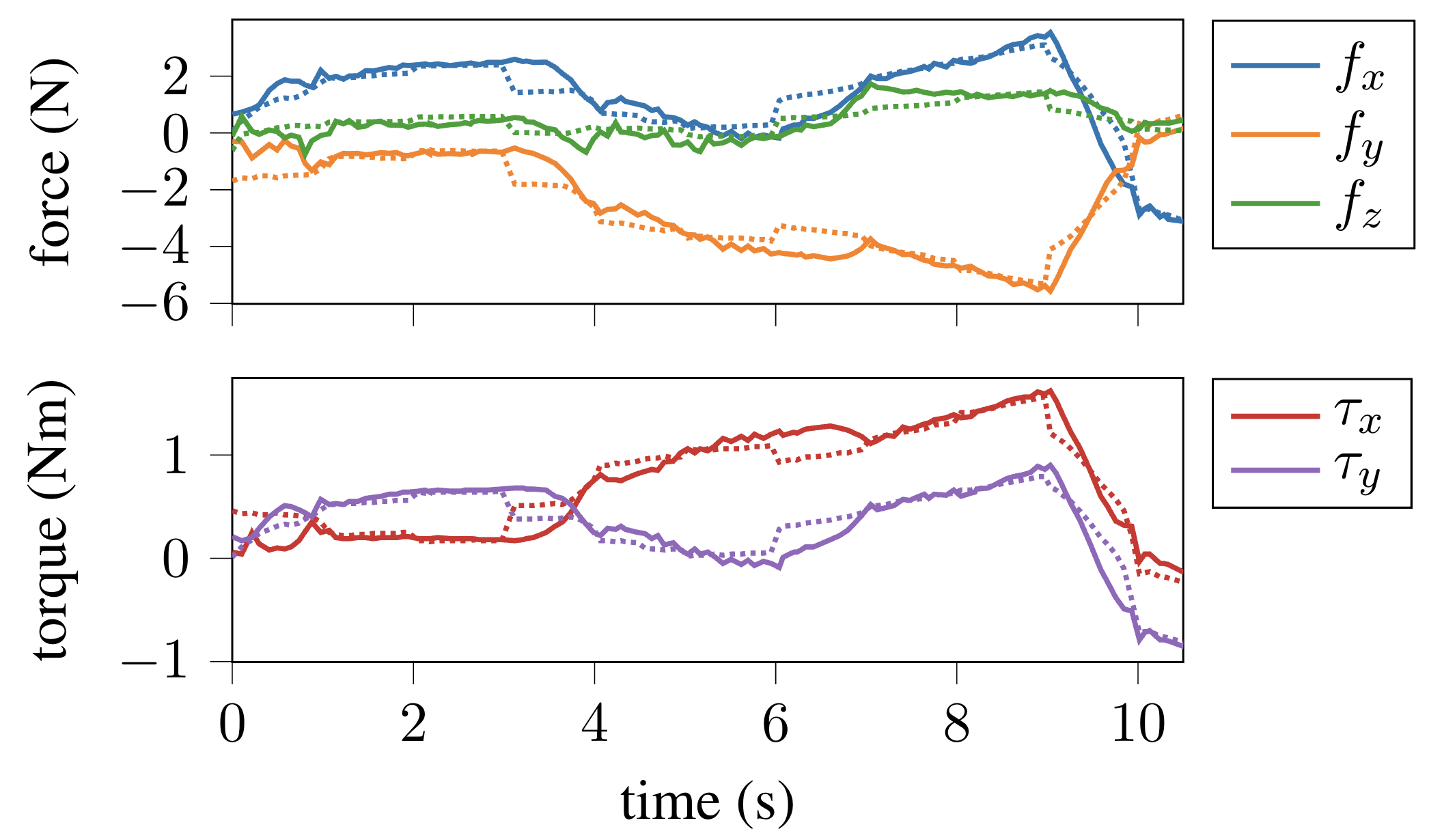
The sim to real gap between our learned model and an experiment. The real force torque sensor data is solid, and the predicted measurements from our learned model are dotted.
With nice agreement between our model and reality, we now use a model-based controller to drive down the force and torque on the connector: $$ \begin{align} \min_u \quad & \color{blue}{\overbrace{\color{black}{ \|\hat{y}\|_2^2 }}^{\color{blue}{\text{minimize force/torque}}}} \color{black}{+} \color{red}{\overbrace{\color{black}{ \lambda \|u - u_{old}\|_2^2 }}^{\color{red}{\text{stay close to previous u}}}} \nonumber \\ \text{st} \quad & \hat{y} = \hat{G} \Omega (q,u) \nonumber \\ & u_{\text{lo}} \leq u - u_{old} \leq u_{\text{hi}} \nonumber \end{align} $$ This is a small convex optimization problem where the solutions can be computed $ < 1$ms. This controller is used to align a set of eight different C13 plugs, where each plug is inserted with a scripted insertion, after which a calibration sequence is performed to learn the model, followed by a controlled insertion.
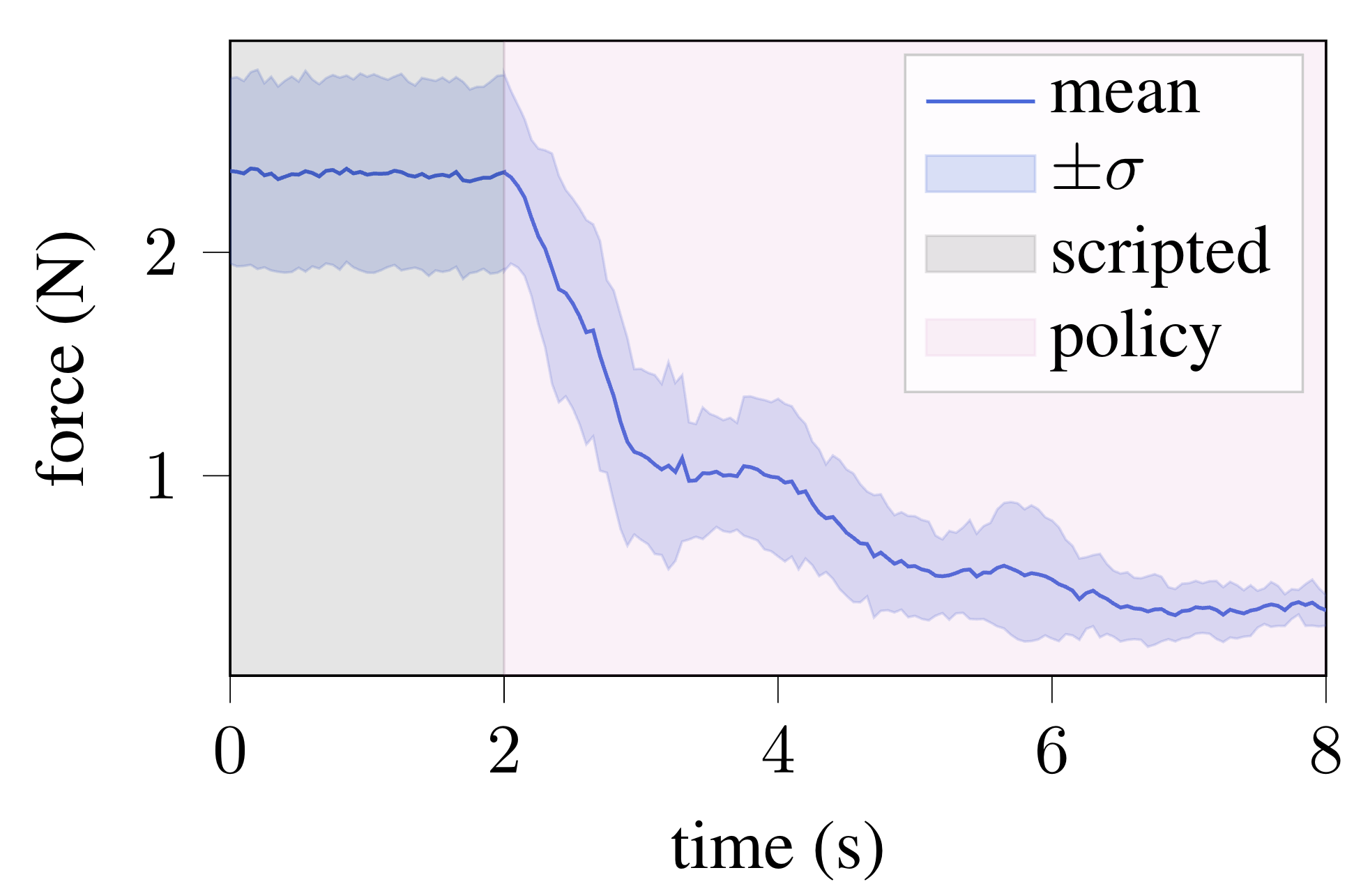
Magnitude of the force on the plug in the XY axis during insertion of eight different plugs. The scripted insertion leaves a constant force on the plug, after which the policy is used to reduce the force on the connector